GOAL SEEK

Goal Seek is a powerful feature in Excel that allows you to find the input value needed to achieve a desired result in a formula. It's particularly useful for performing reverse calculations when you know the outcome you want but are uncertain about the input required to achieve it.

Here's how to use Goal Seek in Excel:

1. **Setup your Excel Spreadsheet**: 
   - Enter your formula in a cell that calculates the result based on certain input values.
   - Enter initial values for the inputs.
   - Enter the desired result in a separate cell.

2. **Navigate to the Goal Seek Feature**:
   - Go to the "Data" tab in the Excel ribbon.
   - Look for the "Forecast" group.
   - Click on "What-If Analysis".
   - Select "Goal Seek" from the drop-down menu.

3. **Configure Goal Seek**:
   - In the Goal Seek dialog box, you'll see three input fields:
     - "Set cell": This is the cell containing the formula you want to adjust.
     - "To value": Enter the desired result you want to achieve.
     - "By changing cell": This is the cell containing the input value you want Excel to adjust.
   - Click OK after setting these parameters.

4. **Review the Results**:
   - Excel will attempt to find the input value needed to achieve the desired result.
   - If it succeeds, it will update the input cell with the new value.
   - If it cannot find a solution, it will display a message indicating that it was unable to achieve the desired result.

5. **Review and Adjust**:
   - After Goal Seek completes its calculation, review the adjusted input value.
   - Make any necessary adjustments to your spreadsheet based on the new input value.

Here's a simple example to illustrate Goal Seek:

Suppose you have a loan repayment calculation where you want to determine the monthly payment needed to pay off a loan of $10,000 in 5 years at an interest rate of 5% per annum.

1. Enter the loan amount, interest rate, and loan term in cells A1, A2, and A3, respectively.
2. Use the PMT function in cell A4 to calculate the monthly payment required: `=PMT(A2/12, A3*12, -A1)`.
3. Enter the desired result (e.g., 200) in a separate cell (e.g., B1).
4. Use Goal Seek to find out what monthly payment is needed to achieve the desired result.
   - Set cell: B1 (the cell containing the desired result).
   - To value: 200 (the desired monthly payment).
   - By changing cell: A4 (the cell containing the monthly payment formula).
5. Excel will calculate and update the monthly payment in cell A4 to achieve the desired result in cell B1.

SUMIFS FORMULA

The SUMIFS function in Excel allows you to sum values based on multiple criteria. It's useful for situations where you need to sum data based on conditions in multiple columns. Let's say you have a table of student payments and you want to calculate the total payment amount for a specific fee type and a specific student ID. Here's how you can use the SUMIFS function:

Suppose you have the following data in your "Payments" sheet:

| Student ID | Payment Date | Fee Type     | Amount |
|------------|--------------|--------------|--------|
| 101        | 2024-04-01   | Tuition Fee  | $500   |
| 102        | 2024-04-02   | Tuition Fee  | $500   |
| 101        | 2024-04-03   | Lab Fee      | $100   |
| 102        | 2024-04-04   | Lab Fee      | $100   |
| 101        | 2024-04-05   | Transportation Fee | $50   |

And let's say you want to calculate the total payment amount for Tuition Fee made by student ID 101.

You can use the SUMIFS function as follows:

```excel
=SUMIFS(D:D, A:A, 101, C:C, "Tuition Fee")
```

Explanation:
- `D:D` is the range of amounts you want to sum.
- `A:A` is the range of student IDs.
- `101` is the criteria for student ID.
- `C:C` is the range of fee types.
- `"Tuition Fee"` is the criteria for fee type.

This formula will sum the values in column D (Amount) where the Student ID is 101 and the Fee Type is "Tuition Fee".

In this example, the result would be $500, as student ID 101 made a payment of $500 for the Tuition Fee.

To create an automatic serial number formula in Excel

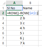
     Type formula in A2 cell
     =row()-row($A$1) 
     
     - Replace `A2` with the first cell where you expect data to be entered. This formula assumes that if there is data in cell A2, then the serial number should start from the second row. If your data starts from a different cell, adjust the reference accordingly.
     - The `ROW()` function returns the current row number.
     - `-1` is subtracted to offset the header row, if any.
     - The `IF` function checks if the reference cell (`A2` in this case) is not empty. If it's not empty, it returns the current row number minus 1 (to account for the header row), otherwise, it returns an empty string.
   
4. **Press Enter**: After entering the formula, press Enter to apply it to the selected cell.

5. **AutoFill**: Click on the bottom right corner of the cell with the formula (the fill handle) and drag it down to fill the formula for the rest of your data. Excel will automatically adjust the references as needed.

Now, whenever you enter data in the specified column (e.g., column A), the serial numbers will be generated automatically in the adjacent column.

This formula ensures that serial numbers are generated dynamically as you enter data, and they adjust automatically if rows are inserted or deleted.

Prevent Duplicate Entry 

It has been seen many times in Excel that while entering data, there are many duplicate entries, due to which we have to sit for hours and find duplicate data, and face difficulties. In such a situation, we want that there should not be duplicate data type, for which we have Data Validation Command in Excel which is present in Data Tools group of Data Tab. With the help of Data Validation or countif formula, you can avoid writing duplicate data in excel. For example, suppose that you have a user's Roll Number, Account Number, Aadhar Number, Registration Number etc. If you want to avoid writing duplicate then you can use Data Validation or countif formula.

I have a data, in which I am entering the data of Name and Roll Number and I want that there should be no Duplicate Value of Roll Number, so I will follow the below steps and prevent Duplicate Entry from being typed in my data.

Steps to stop duplicate value entry in excel

• Click on the heading of the column on which you want to prevent duplicates. Suppose you click on B column, whose B column will be selected.
• Click on Data tab
• Click on Data Validation
• Inside the settings tab, click on the Allow list and select custom.
• Now you will get a text box of a formula in which the following formula has to be typed –

             =COUNTIF(B:B,B1)=1

• Click on ok button

Excel में कई बार देखा गया है कि डाटा एंट्री करते समय बहुत सारे duplicate entry हो जाते है, जिसेसे हमें घंटो बैठ कर डुप्‍लीकेट डाटा को ढुँढना पड़ता है, और कठिनाईयों का सामना करना पड़ता है। ऐसे स्थिति में हम चाहते है, कि डुप्‍लीकेट डाटा टाईप न हो जिसके लिए हमें Excel में Data Validation Command जो Data Tab के Data Tools group में मौजुद है। Data Validation or countif formula की मदद से excel में duplicate data लिखने से बच सकते है। जैसे मान लिजिए कि आप किसी प्रयोक्‍ता का Roll Number, Account Number, Aadhar Number, Registration Number etc. duplicate लिखने से बचना चाहते है तो आप Data Validation or countif formula का प्रयोग कर सकते है।

मेरे पास एक डाटा है, जिसमे Name और Roll Number की डाटा एंट्री कर रहा हूँ और मैं चाहता हुँ  कि कोई Roll Number की Duplicate Value न हो इसीलिए मैं नीचे दिए steps को follow करूंगा और मेरे डाटा मे Duplicate Entry को type होने से रोकूँगा।

Steps to stop duplicate value entry in excel

• उस column को select कीजिये जिसमे duplicate data को type होने से रोकना हैं। जैसे कि मैंने Column B पर click किया, जिससे B Column पुरा select हो जायेगा। 
• अब आपको Data tab पर click करना है।
• उसके बाद में Data Validation पर click करना है।
• उसके बाद आपके सामने data validation dialog box open हो जायेगा।
• जिसमें settings tab के अंदर Allow list पर click करके custom को select करना है।
• अब आपको एक formula का text box मिलेगा जिसमें निचे दिए गए formula  को टाईप करना है –

=COUNTIF(B:B,B1)=1

• Ok button पर click करे ।

How to Use Print Title In Excel (Repeat the top row on every page in Excel)

The Print Title command is in the Page Setup group of the Page Layout tab. With the help of this command, we can print the row headings or column headings of the first page in Excel on many pages.

              So in today's blog, we know how to print row heading and column heading on every page in Excel?

              Let's understand this with a good example. Suppose you have an Excel sheet with lots of records spread over more than one page. And you want the Row Heading or Column Heading on the first page to be printed on each page. For this you have to follow our steps given below.

• Start excel and type data

• Click on page layout tab
• Click on print titles
• Click on sheet tab
• Click on row to repeat at top box
• Now click on top headings or row of your data
• Click on ok button
• Press CTRL + P (Print Preview/ Print)

Print Title command Page Layout tab के Page Setup group में होते है। इस कमाण्‍ड की सहायता से हम Excel मे पहले पेज के row headings or column heading को बहुत सारे पेज पर प्रिन्ट कर सकते है ।

              तो आज के इस ब्लॉग मे हम Excel  में row Heading  और column heading  को हर एक पेज पर  कैसे  प्रिंट करे ये जानते है?  

              आईए इसे एक बढि़या सा उदाहरण के साथ समझते है मान लिजिए कि आपके पास एक Excel sheet है जिसमे बहुत सारे रिकॉर्ड है जो एक से ज्‍यादा पेज पर है। और आप चाहते है कि पहले पेज पर जो Row Heading or Column Heading  है वो हर एक पेज पर प्रिंट हो। इसके लिए आपको नीचे दिए हमारे steps को follow करना होगा ।

• सबसे पहले आप Excel  open करे और डाटा को टाईप कर ले Row Heading में ।

• Page Layout Tab पर click करे
• Print Titles पर click करे
• Sheet tab पर click करे
• Row to repeat at top box  पर click करे
• फिर excel sheet में सबसे उपर row Title या Heading Row  को click करे
• OK button पर click करे
• Keyboard से CTRL + P key को दबाकर print देख ले कि headings सारे page पर print हो रहे है कि नहीं

Note - इसी तरह आप चाहे तो column heading  को भी हर पेज पर repeat कर सकते है बस आपको उस COLUMNS TO REPEAT  AT LEFT करके आप first Column को select करके print preview देख सकते है।

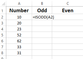
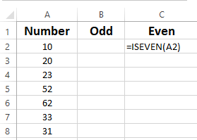
Ms - Excel में बने डाटा में ODD Number के सामने True और EVEN Number के सामने False Or EVEN Number के सामने True और ODD Number  के सामने False  को दिखाने के लिए आपको अमित सर के बताये गये formula को follow करना होगा।

Ms - Excel में बने डाटा में अगर किसी सेल में नंबर के साथ-साथ text भी type है तो अगर आप Sum करना चाहते है तो  आपको अमित सर के बताये गये formula को follow करना होगा ।

1. सबसे पहले सेल को सेलेक्ट करे
2. Press CTRL + 1
3. 
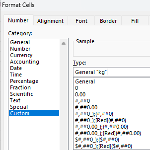
4. Ok button
5. Then use sum formula